Boundary Attention
Learning curves, corners, junctions and grouping
1Google Research 2Harvard University
We introduce a form of local attention that infers unrasterized boundaries—including contours, corners and junctions—from the bottom-up.

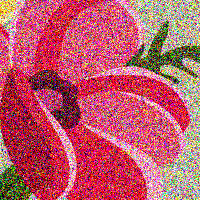


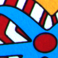

We introduce a lightweight, bottom-up model that infers color-based boundaries with high-precision. Output boundaries are represented by a field of embeddings that encode three-way partitions and associated windowing functions of every stride-1 patch in an image. This output can express a variety of boundary elements, including contours, thin bars, corners, T-junctions and Y-junctions. It expresses them without rasterization, and so with unlimited resolution.
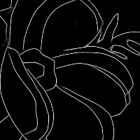
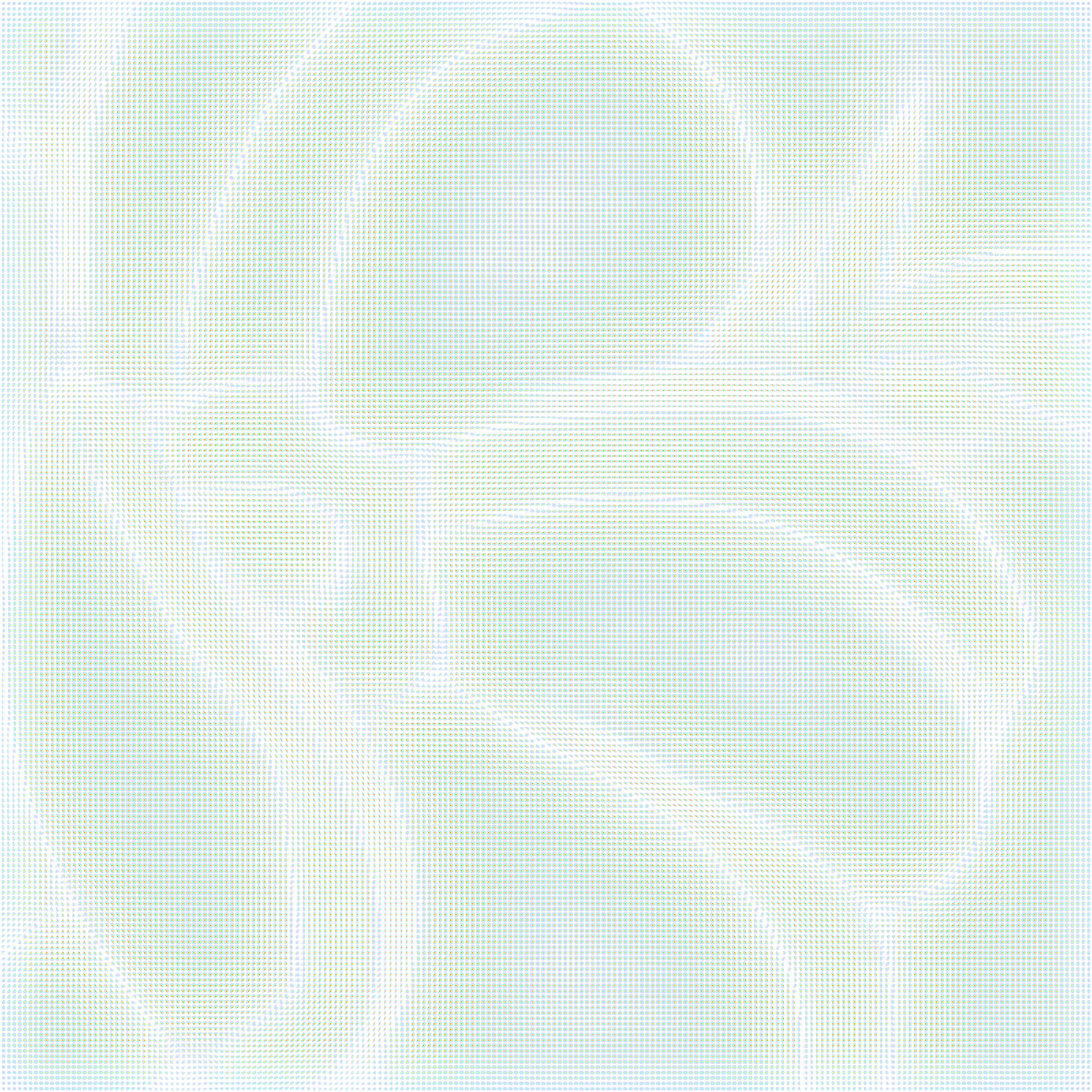
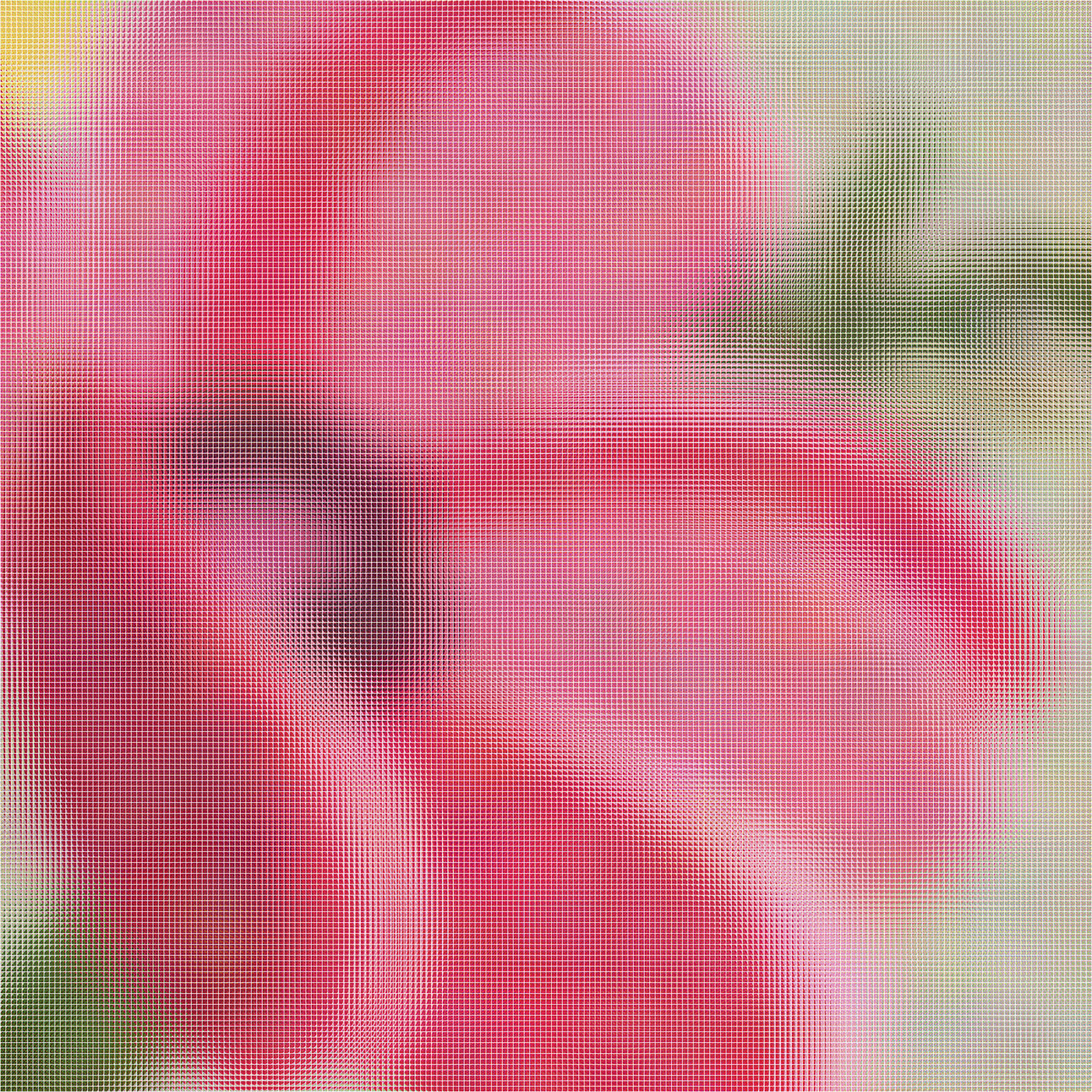
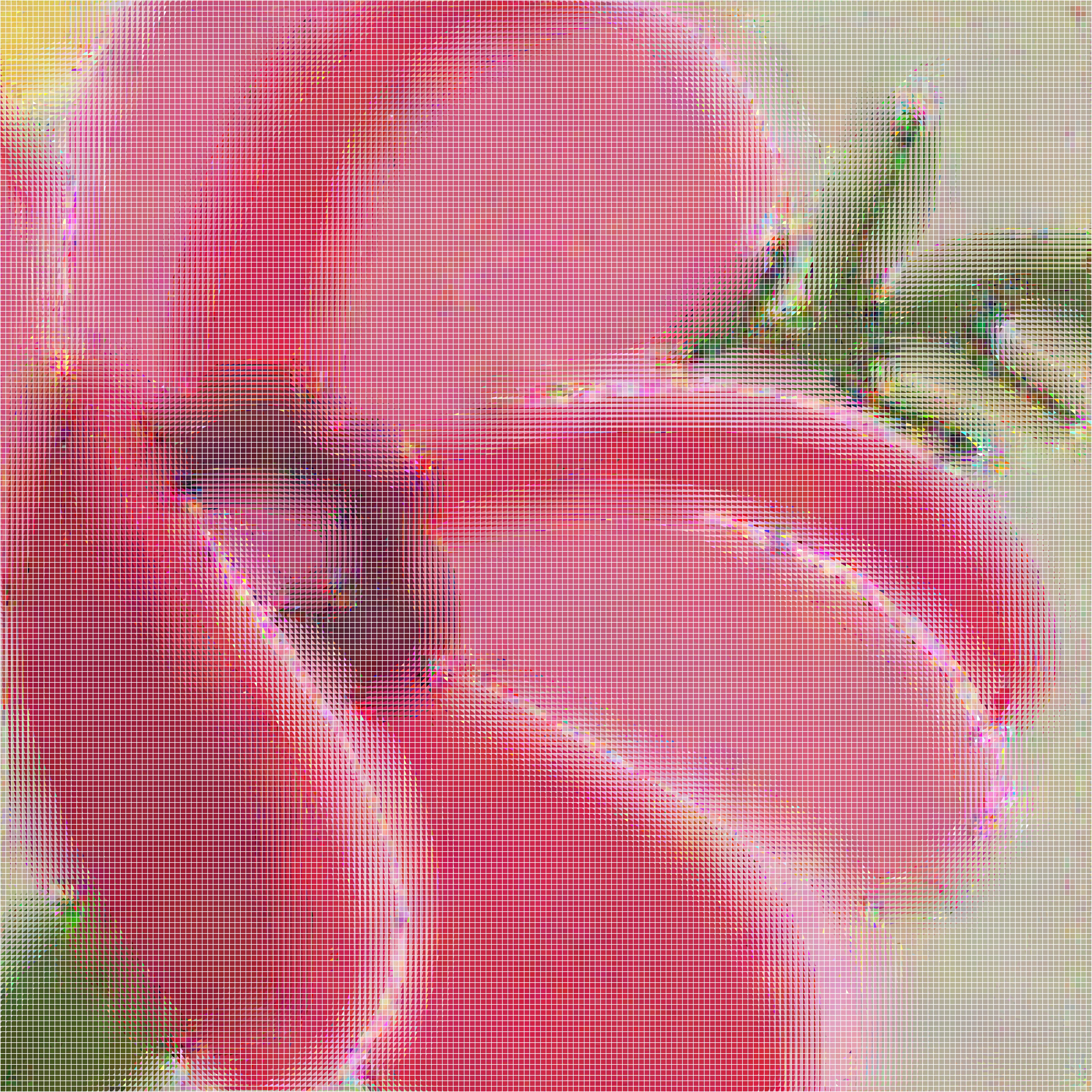
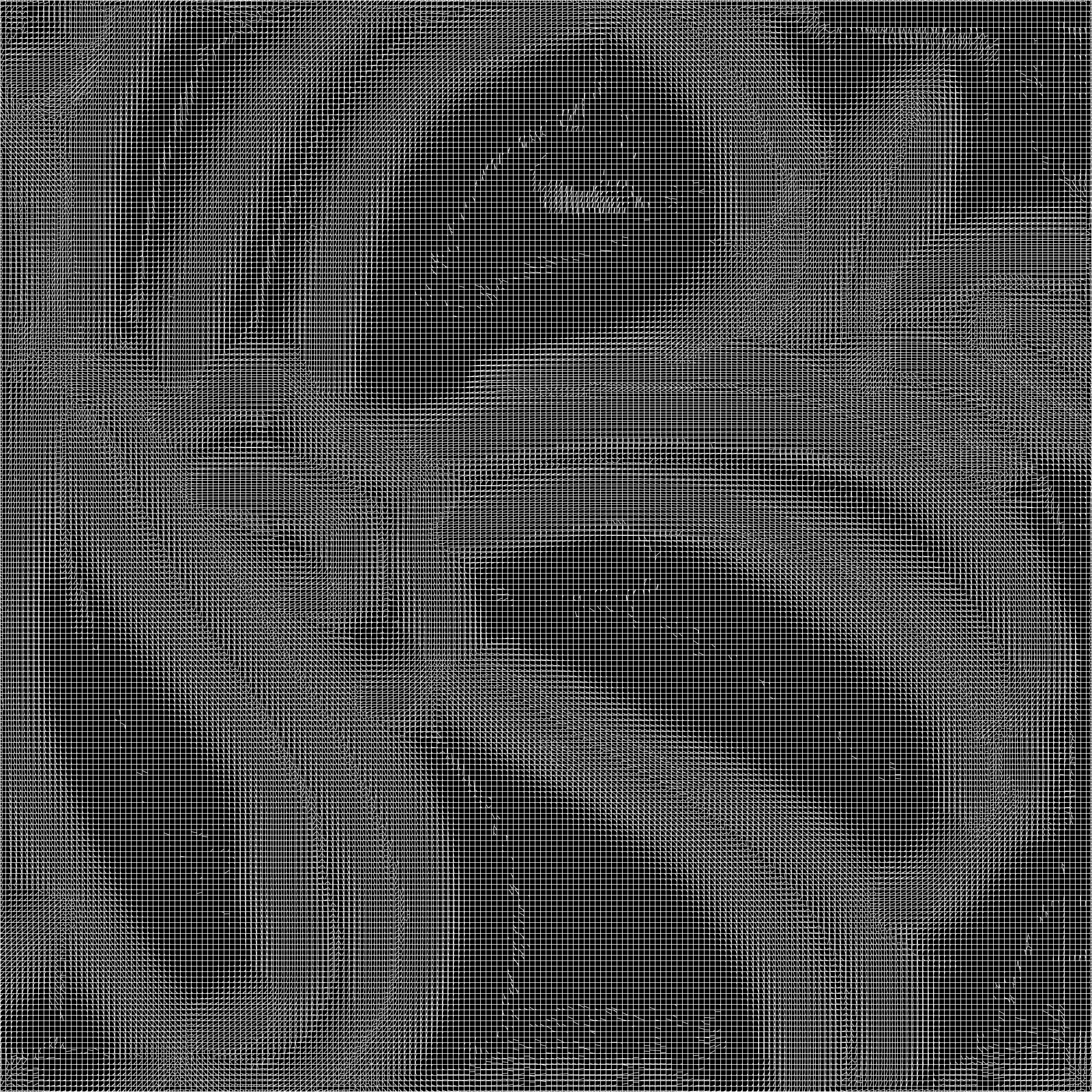
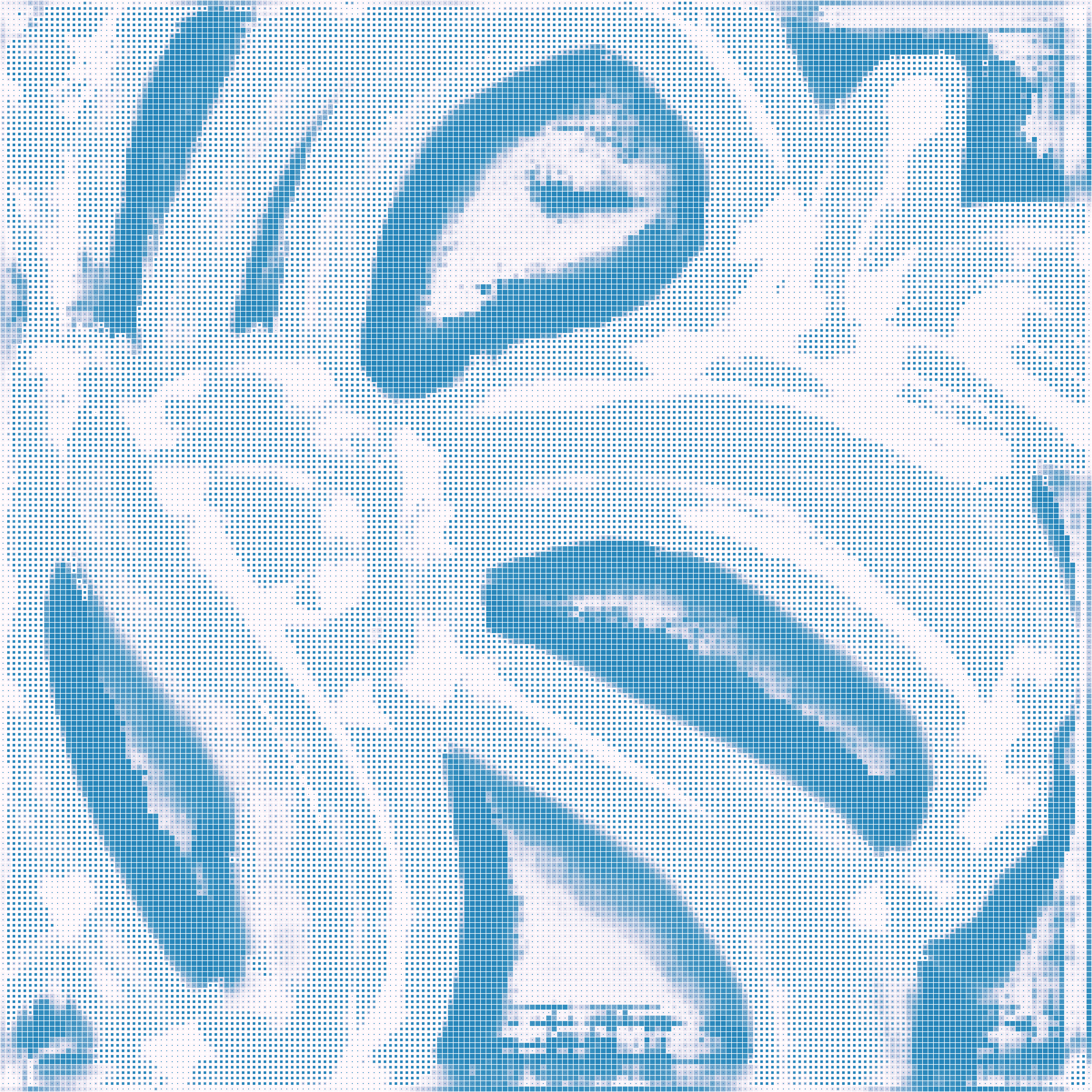
The figure's bottom row shows these outputs as you scroll, with each patch's partition visualized by its boundaries, its segment colors, and its associated windowing function. Various global accumulations of these overlapping patches lead to the pixel-resolution output maps in the figure's top row: a boundary-aware smoothing of the input colors, a global boundary map, and the spatial affinities between each pixel and all of its neighbors.
The core of our model is a specialized form of neighborhood self-attention that we call Boundary Attention. We find that we can train it to a useful state using very simple synthetic images, which suggests it has an inductive bias for boundaries. Also, since all of its operations are local and bottom-up, we can train it on small images and then deploy it at any image size and aspect ratio.
Model Details
Overview

At a high level, our model learns a field of special geometric embeddings for every patch in an image. The input image unfolds into stride-1 patches, and boundary attention operates iteratively on their embeddings to produce for each patch: $(\bf{i})$ a parametric three-way partitioning, and $(\bf{ii})$ a parametric windowing function that defines its effective patch size. This output field implies a variety of global maps, shown in clockwise order: a boundary-aware smoothing of the input colors; an unsigned boundary-distance map; a boundary map; and a map of spatial affinities between any query point and its neighbors.
Representing Per-Patch Boundaries in Junction Space
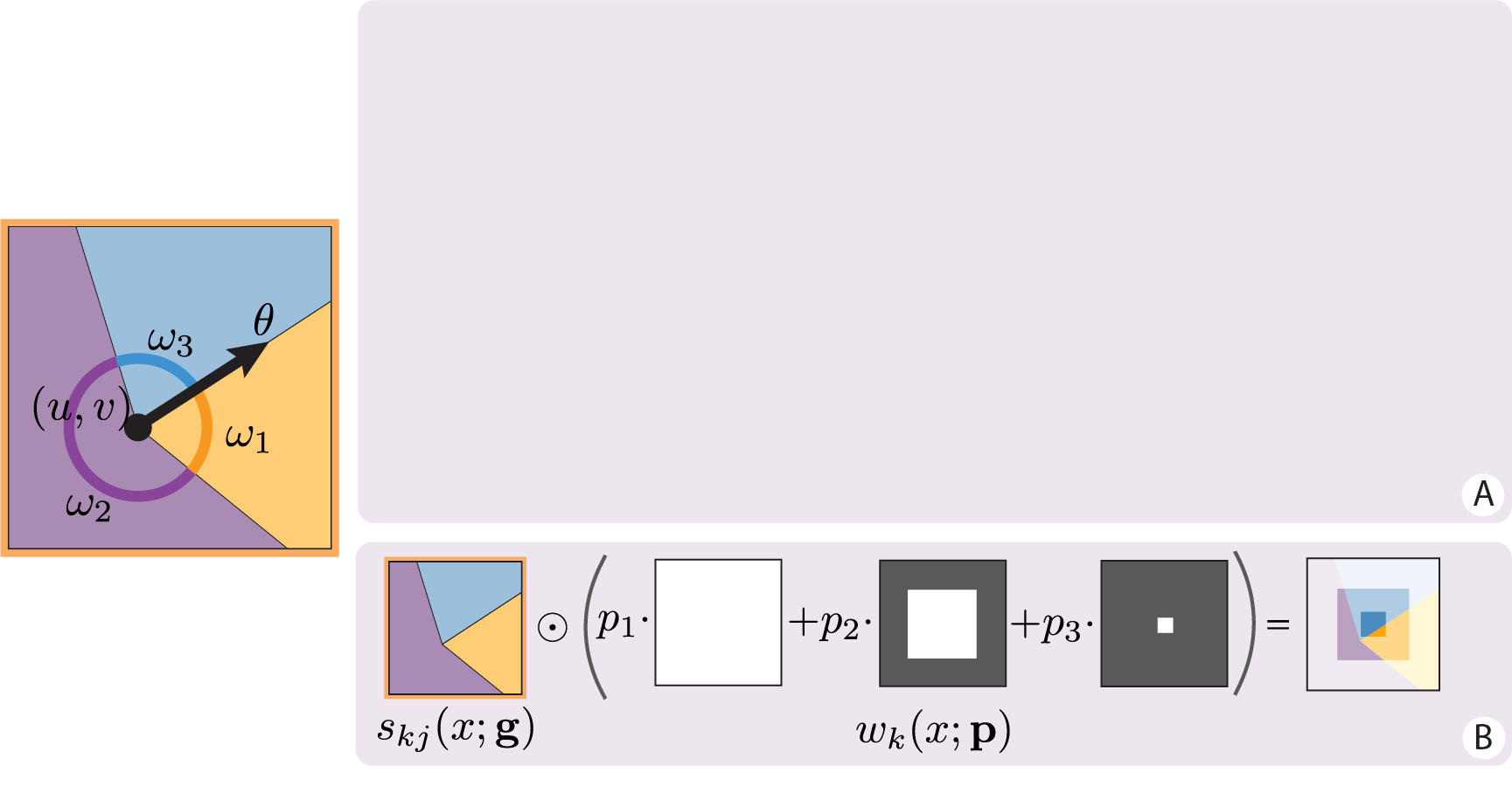
We describe each patch's three-way partition—referred to as a junction—by parameters $g \in \mathbb{R}^2 \times \mathbb{S}^1 \times \Delta^2$, comprising a vertex $(u,v)$, orientation $\theta$ and relative angles $(\omega_1,\omega_2,\omega_3)$ that sum to $2\pi$.
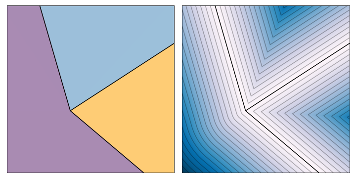
Walks in junction space are spatially smooth and can represent a variety of local boundary patterns, including uniformity (i.e., absence of boundaries), edges, bars, corners, T-junctions and Y-junctions. These local boundary patterns can be visualized by moving the slider bar in $\text{A}$. To the right, we show each junction's implied unsigned distance map.
Our method also associates each junction with a learned spatial windowing function. In $\text{B}$, we show how a junction is modulated through its windowing function. The windowing parameters $\mathbf{p} = (p_1, p_2, p_3)$ are convex weights over a dictionary of binary pillboxes. This modification allows our model to vary boundaries according to local context in order to represent both fine and coarse details.

Boundary Attention
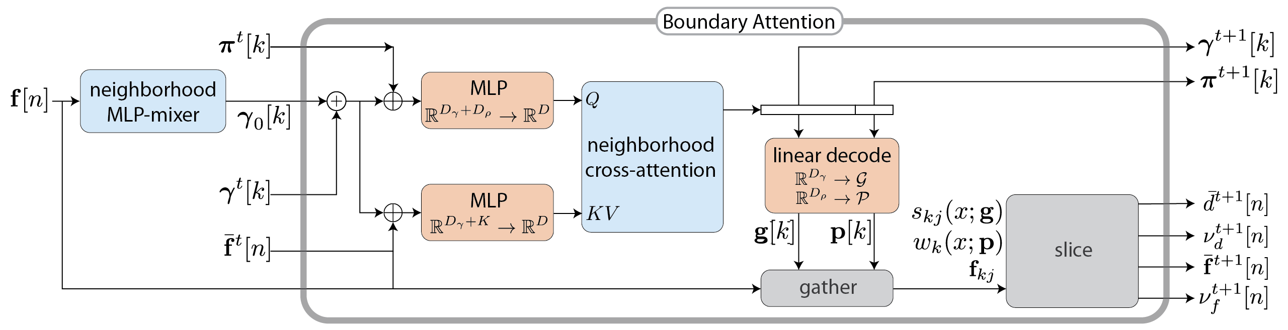
Our model produces the output vector fields by learning an embedding $\gamma$ of junction parameters $g$ and iteratively updating the pixel-resolution field of these embeddings $\gamma[n]$ using a specialized variant of neighborhood dot-product attention. It simultaneously updates a field of embedded windowing functions $\pi[n]$.
The model uses eight iterations of boundary attention in total, with some weight-sharing across iterations. It includes two parameter-free operations—gather and slice—that perform rasterizations and foldings which are specific to junctions. The entire model is invariant to discrete spatial shifts and so applies to inputs of any size. It is also fairly compact, with only 207k parameters.
Training Data
We find it sufficient to train the model on simple synthetic data, consisting of overlapping circles and squares. Each shape is uniformly colored, and the images are "augmented" during training by perturbing them with varying types and amounts of noise.
We train our model to predict the unsigned distance function for the true visible boundaries, which is known up to machine precision.
Emergent Properties
Generalization to Natural Images
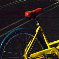
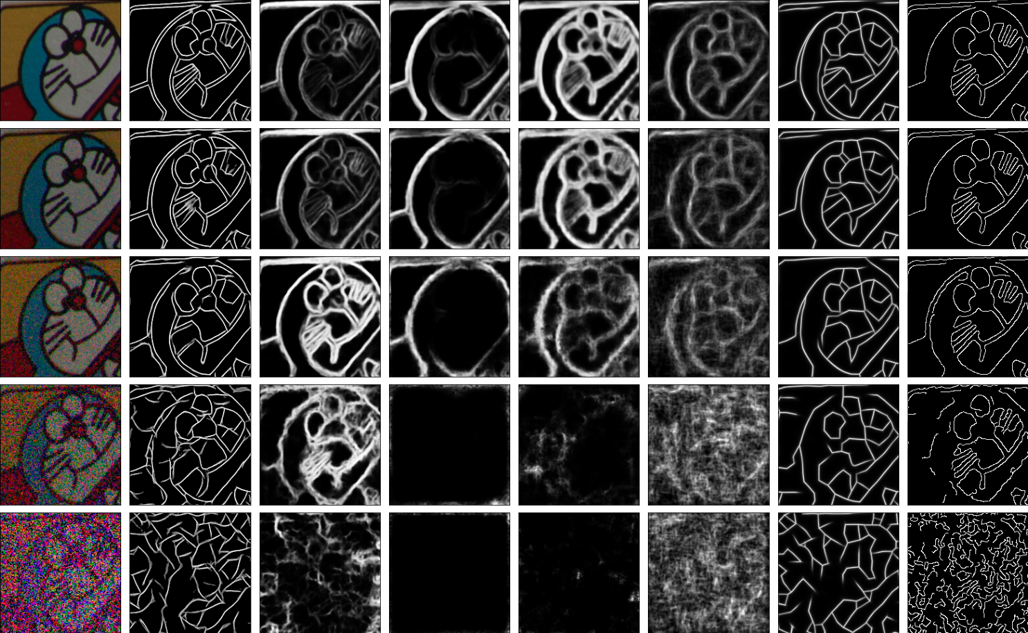
Despite being trained on very simple synthetic data, the model provides reasonable boundaries for natural images. The boundaries are combinations of fine geometric structures and coarse ones, and they are quite stable across exposure conditions that have varying amounts of sensor noise. The qualitative properties of our model's boundaries are somewhat different from those of classical bottom-up methods and from those of learned, end-to-end models that are trained to match human annotations. Its boundaries are based purely on color and so include finer structures than those of end-to-end systems. And its inference of local window sizes allows it to produce both fine and coarse structures, unlike many classical bottom-up methods that use a single patch-size everywhere.
Visual Comparison
More Examples
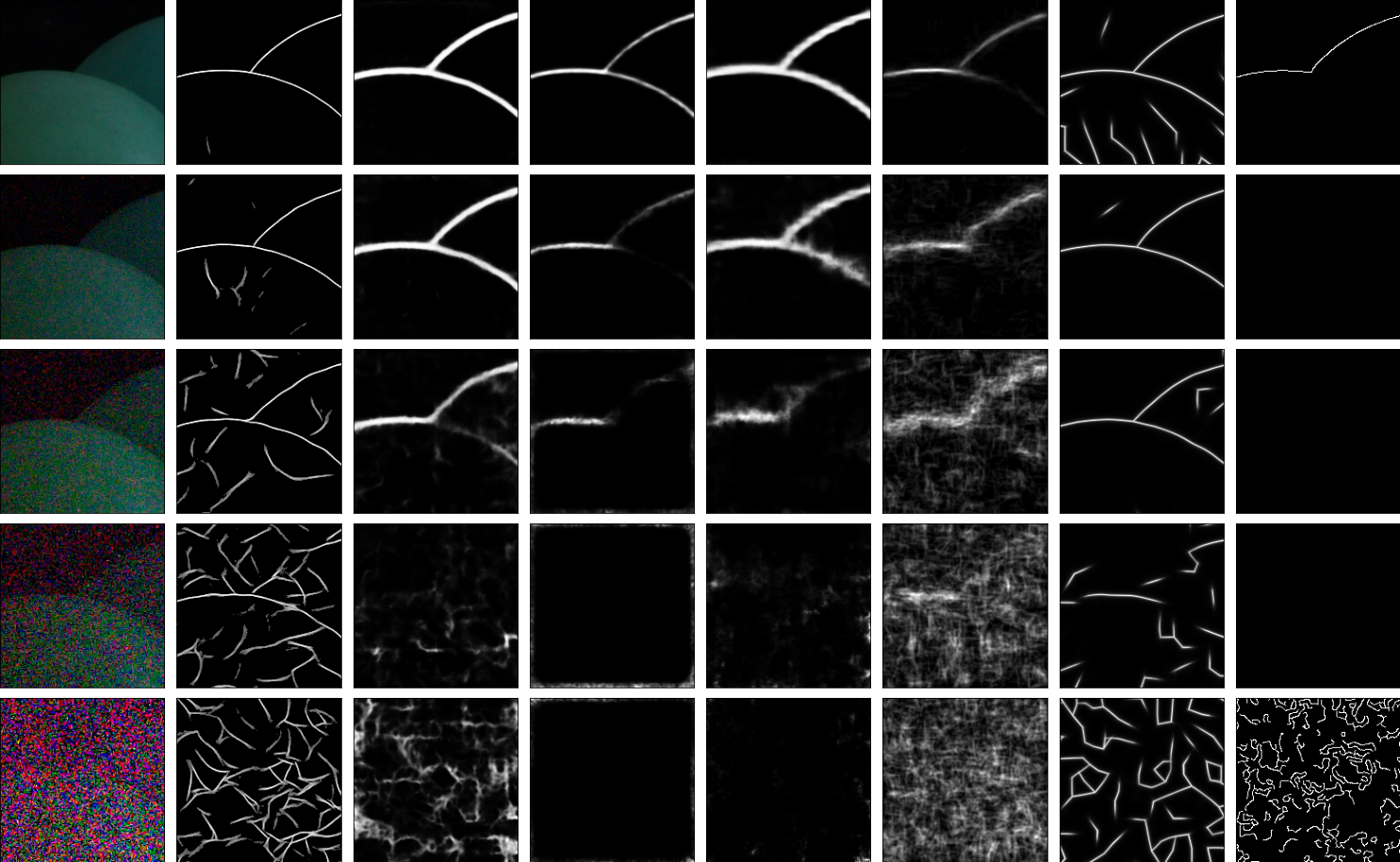
Low Light Boundary Detection
Our model produces crisp boundaries for photographs with high levels of sensor noise. Its success is in part due to the inferred local windowing functions. In general, smaller windows are good for recovering fine structures in low-noise situations but can cause false boundaries at high noise levels. Conversely, larger windows provide more resilience to noise but cannot recover fine structures. By automatically inferring a window for every patch, our model combines the benefits of both.
Output Boundaries
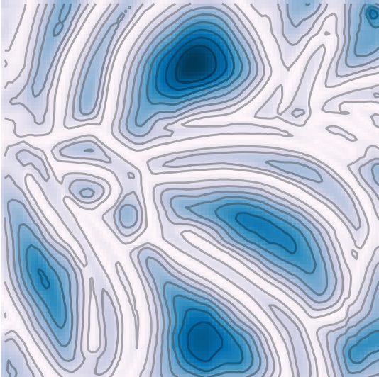
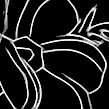
The output junction $g[n]$ at each pixel $n$ implies an unsigned distance map over the windowed patch surrounding it. To get a global unsigned distance map for the image, we simply compute the pixel-wise average (“slice”) of the overlapping patches. We visualize this global map by applying a non-linearity to amplify its zero-distance set, and we call this the output boundary map. This definition of output boundaries is unrasterized and so can be rendered at any resolution and thickness. Below, we render them at super-resolution (left) and change their thickness by adjusting our non-linearity's parameter (right).


Evolution of Boundaries
At any point during the iterations, we can probe the intermediate junctions and their implied boundaries. We find they are exploratory and unstructured during early iterations, and become spatially-consistent during later ones.
Output Spatial Affinities

Another way to visualize our output $g[n]$ is through the pairwise affinities they imply. We compute the spatial affinity between any query pixel $n$ and its neighbors $n'$ as the normalized sum of junction-segments that contain $n$. These spatial affinities respect boundaries, and they serve as the filtering kernels that convert the noisy input image colors to the output smooth ones.
Embedding of Junction Space
We also find that the model's learned embedding of junction space is smooth. The top row of this figure visualizes equally-spaced samples, in the Euclidean sense, of embeddings $\gamma_i$ from starting point $\gamma_a$ to $\gamma=0$ and to ending point $\gamma_b$. For comparison, the bottom row shows a comparable, analytically-designed interpolation in junction space $\mathbb{R}^2 \times \mathbb{S}^1 \times \Delta^2$. Interestingly, the model learns to associate $\gamma=0$ with nearly-equal angles and a vertex close to the patch center.
BibTeX
@article{mia2023boundaries,
            author    = {Polansky, Mia Gaia and Herrmann, Charles and Hur, Junhwa and Sun, Deqing
                        and Verbin, Dor and Zickler, Todd},
            title     = {Boundary Attention: Learning to Find Faint Boundaries at Any Resolution},
            journal   = {arXiv},
            year      = {2023},
            }
Contact Info
Always happy to chat at miapolansky at g.harvard.edu.